# Let's check the count of filescat("total training cat images:", length(list.files(train_cats_dir)), "\n")cat("total training dog images:", length(list.files(train_dogs_dir)), "\n")cat("total validation cat images:", length(list.files(validation_cats_dir)), "\n")cat("total validation dog images:", length(list.files(validation_dogs_dir)), "\n")cat("total test cat images:", length(list.files(test_cats_dir)), "\n")cat("total test dog images:", length(list.files(test_dogs_dir)), "\n")
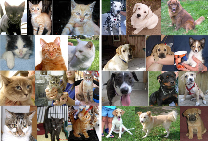
So we have 2,000 images for training, 1,000 for validation and 1,000 for testing. Each of the splits contain the same number of samples from each class thus this is balanced binary-classification problem which means classification ‘accuracy’ will be an appropriate measure of success.
Set Image Generators
We need to convert the data from PNG images to integer values between [0,1]. Here, keras provides us with image_data_generator() which automatically turns image files on disk into batches of pre-processed tensors.
The generators yields batches of 150x150 images of shape (20,150,150,3) and binary labels of shape (20) . ‘20’ because we specify batch_size = 20 i.e. 20 samples in each batch. The generator yields these batches indefinitely because it loops endlessly over the images in the specified folder. Here, for training we have 2000 images, read in batch-wise a 100 times.
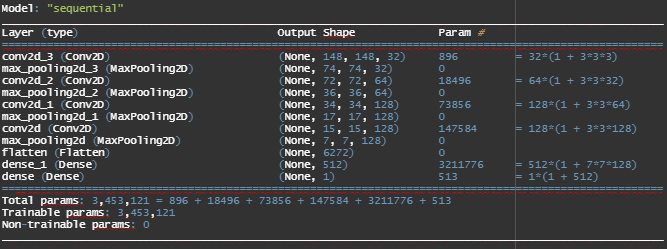
Our input images are of dimension 150 by 150 pixels. These images are coloured thus, we have 3 channels for RGB. As we go deeper into the network, the feature map reduces from 148x148 to 7x7 and depth increases from 32 to 128.
Now, we want the output to be a single probability - thus we have 1 output neuron with sigmoid activation. Also, because we end up with a single sigmoid unit at end - we use binary cross entropy in the compilation step.
We use fit(<train_generator>, <steps_per_epoch>, <epochs>, <validation_data_generator>, <validation_steps>).
train_generator - provides batches of inputs and targets indefinitely (as we saw above)
steps_per_epoch - tells the number of samples to draw from the generator before moving on to the next epoch/iteration. Here, we have 2000 training images in batches of 20, so we need 100 steps to cover all images.
epochs = 30 i.e. iterations or number of times the network should run.
validation_data_generator - just like train_generator which yield batches of validation inputs and targets
validation_steps = 50 because we have 1000 images rolled in batches of 20.
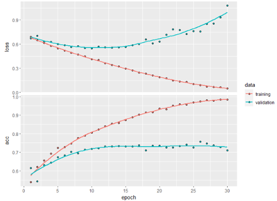
The Training Accuracy increases almost linearly to 100% while the Validation Accuracy stabilises around 70-75%. This clearly indicates that there is a lot of overfitting - one apparent reason being small training sample size of 2000.
One way to deal with over-fitting is to introduce more training data so that there can be better generalisation. This can be achieved by exploiting a technique called Data Augmentation.
Data Augmentation
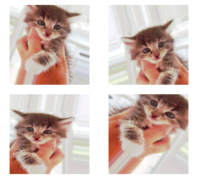
The idea of Data Augmentation is to make small random tweaks and changes to the training images so that we end up with more training data. These random changes or transformations can be :
rotation_range -> rotate image in degrees (0-180)
width_shift_range & height_shift_range -> by what fraction of total width/height should the picture be randomly translated vertically or horizontally
shear_range -> applying shearing transformation i.e. change shape of image (angle in radians)
zoom_range -> zooming in/out pictures in the range [1-z, 1+z] where we specify ‘z’
horizontal_flip -> horizontally flip half images - relevant when there is no assumption of horizontal symmetry (for eg real-world pictures)
vertical_flip -> vertically flip half images - FALSE because we need to maintain vertical symmetry e.g. head -> torso -> legs
fill_mode -> strategy used for filling in newly created pixels, which can appear after a rotation or a width/height shift.
Code
datagen =image_data_generator(rescale =1/255, rotation_range =40,width_shift_range =0.2, height_shift_range =0.2, shear_range =0.2,zoom_range =0.2, horizontal_flip = T, fill_mode ="nearest")## Looking at the augmented images#(1) create a list of training imagesfnames =list.files(train_cats_dir, full.names = T)#(2) pick one image to augmentimg_path = fnames[[3]]#(3) read in the image and resizes it accordinglyimg =image_load(img_path, target_size =c(150,150))#(4) convert into an array shape (150,150,3)img_array =image_to_array(img)#(5) reshapes to (1,150,150,3)img_array =array_reshape(img_array, c(1,150,150,3))#(6) generate batches of randomly transformed images. augmentation_generator =flow_images_from_data(img_array, generator = datagen,batch_size =1)# note : since generator loops indefinitely, specifying batch_size = 1 tells it to end after reading the 1 image#(7) plotop =par(mfrow=c(2,2), pty="s", mar=c(1,0,1,0))for (i in1:4) { batch =generator_next(augmentation_generator)plot(as.raster(batch[1,,,]))}par(op)
Data Augmentation
New Model Structure
Code
# We also include a dropout layermodel <-keras_model_sequential() %>%layer_conv_2d(filters =32, kernel_size =c(3, 3), activation ="relu",input_shape =c(150, 150, 3)) %>%layer_max_pooling_2d(pool_size =c(2, 2)) %>%layer_conv_2d(filters =64, kernel_size =c(3, 3), activation ="relu") %>%layer_max_pooling_2d(pool_size =c(2, 2)) %>%layer_conv_2d(filters =128, kernel_size =c(3, 3), activation ="relu") %>%layer_max_pooling_2d(pool_size =c(2, 2)) %>%layer_conv_2d(filters =128, kernel_size =c(3, 3), activation ="relu") %>%layer_max_pooling_2d(pool_size =c(2, 2)) %>%layer_flatten() %>%layer_dropout(rate =0.5) %>%layer_dense(units =512, activation ="relu") %>%layer_dense(units =46, activation ="softmax")# compilemodel %>%compile(loss="binary_crossentropy",optimizer=optimizer_rmsprop(learning_rate =1e-4), metrics=c("acc"))# Data Augmentation datagen <-image_data_generator(rescale =1/255,rotation_range =40,width_shift_range =0.2,height_shift_range =0.2,shear_range =0.2,zoom_range =0.2,horizontal_flip =TRUE)test_datagen <-image_data_generator(rescale =1/255)train_generator <-flow_images_from_directory(train_dir,datagen,target_size =c(150, 150),batch_size =20,class_mode ="binary")validation_generator <-flow_images_from_directory(validation_dir, test_datagen,target_size =c(150, 150),batch_size =20,class_mode ="binary")# Train - we incraese the number of epochs to 100!history <- model %>%fit_generator(train_generator,steps_per_epoch =100,epochs =100, validation_data = validation_generator,validation_steps =50)# train accuracy = 82.50% # validation accuracy = 76.20%# we save the model so that we can later load itmodel %>%save_model_hdf5("cats_and_dogs_small_2.h5")
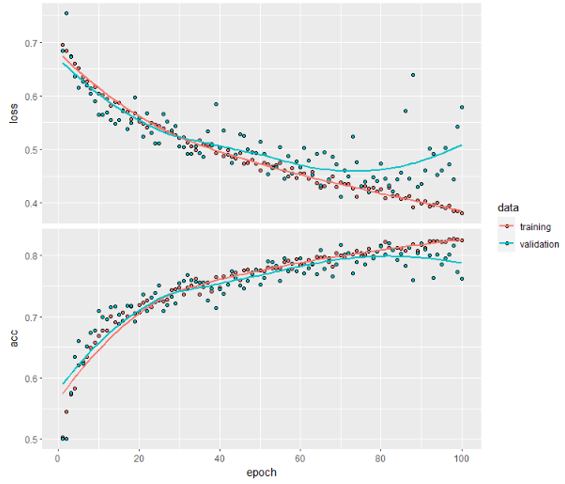
The training and validation accuracy curves increase over epochs quite closely - we are no longer overfitting.
Pre-trained Networks
A Pre-trained network is a saved network which was previously trained on a large dataset. Now, because this network was trained on a large and generic dataset, the spatial-feature hierarchies it has learnt makes it effective for many different computer-vision problems.
For e.g. a network trained on ImageNet dataset which contains 1.4 million labelled images over 1000 different classes, most of which are animals and everyday objects. We can use such a network to identify say furniture/pets in images.
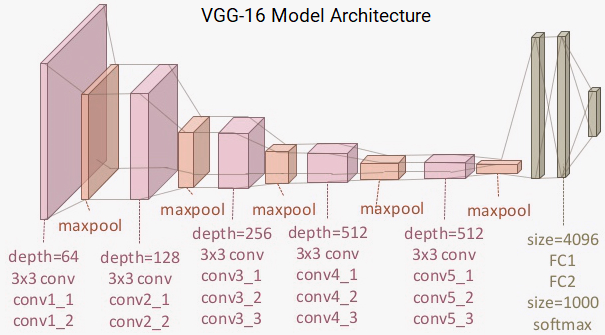
For our cats-vs-dogs problem, we can use the pretrained network called VGG16 which is trained on ImageNet dataset - which contains images of different species of cats and dogs among other animals. Other options provided by Keras are VGG 16, VGG 19, ResNet 50, Inception V3, MobileNet, Xception - all pretrained on ImageNet.
There are 2 ways :- (1) Feature extraction (2) Fine-Tuning
Under Feature Extraction, we use the feature learned by the pre-trained network to extract new features in our samples. Then these extracted features are run through a new classifier (dense network) i.e. we take the convolution base of the pretrained network can run it over our data and train a new classifier on top of the pre-trained network’s output.
Under Fine Tuning, say the pre-trained network has 5 convolution layers, we keep say 4 as it is and train the 5th convolution layer and the classifier. The idea is to retain the learned features of pre-trained network while slightly adjusting the features learnt so that it is more relevant to the dataset we deal with.
Why do we need to train the classifier and not the convolution base?
The representations learnt by the convolution base are generic and thus can be reused while the representations learnt by the classifier are specific to the set of classes on which the model was trained. Also, dense layers get rid of notion of space i.e. it does not contain information about where objects are located in the input image but convolution does contain this information. thus, dense networks are useless for object-location problems.
How generic or re-usable are the pre-trained layers?
As we know, the first few layers of convolution layer extracts local, highly generic feature maps representing features like edges, colour, textures deeper we go, the layers learn more abstract concepts such has “cat ear” or “dog eye”. So if our input dataset differs a lot, we should rely on the first few layers.
(A) Feature Extraction
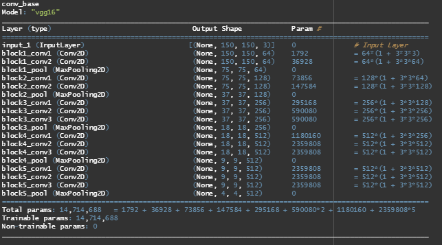
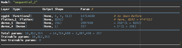
We use the VGG16 network trained on “imagenet” (specified using weights argument), include top = F discards the classifier, input shape specifics what we feed into the network.
Fast Feature Extraction without Data Augmentation - Here, we run the pre-trained convolution base over our dataset, record it’s output and then feed this to a dense classifier. Advantage - computationally cheaper and faster BUT does not allow data augmentation.
Feature Extraction with Data Augmentation - involves running the entire convolution base with the classifier end to end on the inputs.
Method 1 : Fast Feature Extraction without Data Augmentation
Code
batch_size =20datagen <-image_data_generator(rescale =1/255)extract_features =function(directory, sample_count){# empty array for inputs of shape (2000,4,4,512) because the conv base # output is of shape (4,4,512) features =array(0, dim=c(sample_count, 4,4,512)) # empty array for labels labels =array(0, dim=c(sample_count))# generator to read in training data when training directory is specified # in batches of 20 while resizing them to [0,1] generator =flow_images_from_directory(directory = directory, generator = datagen, target_size =c(150,150), batch_size = batch_size, class_mode ="binary") i =0while(TRUE){ batch =generator_next(generator) inputs_batch = batch[[1]] labels_batch = batch[[2]] features_batch = conv_base %>%predict(inputs_batch)# to extract features, we use predict() i.e. we run the convolution base # over our own input images# predict() command outputs the feature maps of (4,4,512) index_range = ((i*batch_size)+1):((i+1)*batch_size) features[index_range,,,]= features_batch labels[index_range] = labels_batch i = i +1if(i*batch_size >= sample_count)break# because generators yield data indefinitely in a loop, we must break # after every image has been seen once# i.e. after i*batch_size >= 2000 we stop loop for reading in training images }list(features=features, labels=labels)}train =extract_features(train_dir, 2000)validation =extract_features(validation_dir, 1000)test =extract_features(test_dir, 1000)# now we need to reshape from (4,4,512) to (2000, 8192) i.e. flatteningreshape_features <-function(features) { array_reshape(features, dim =c(nrow(features), 4*4*512)) }train$features <-reshape_features(train$features)validation$features <-reshape_features(validation$features)test$features <-reshape_features(test$features)
Training is very fast, because you only have to deal with two dense layers-an epoch takes less than one second even on a CPU.
Training Accuracy Plots
We achieve a Training accuracy = 97.70% and a Validation accuracy = 90.1% which is much better than earlier models we trained from scratch. However, the plots indicate that there is overfitting in spite of using drop-out with a fairly large rate. This is because the training sample size is small. We need to use data augmentation.
Method 2 : Feature Extraction with Data Augmentation
CAUTION : Before we compile and train the model, it is very important to freeze the convolutional base. Freezing a layer or set of layers means preventing their weights from being updated during training. If we do not do this, then the representations that were previously learned by the convolutional base will be modified during training.
Code
cat("This is the number of trainable weights before freezing","the conv base:", length(model$trainable_weights), "\n")freeze_weights(conv_base)cat("This is the number of trainable weights after freezing","the conv base:", length(model$trainable_weights), "\n")
Earlier -> This is the number of trainable weights before freezing the conv base: 30
Now -> This is the number of trainable weights after freezing the conv base: 4
Now, only weights from the 2 dense layers will be trained i.e. a total of 4 weight tensors: 2 per layer (the main weight matrix and the bias vector)
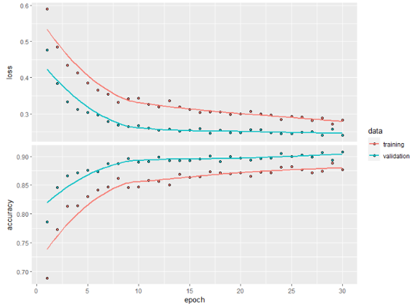
We end up with a Training accuracy = 87.70% and Validation accuracy = 90.80% which is better because we are no longer overfitting. The training and validation error curves fall together, exponentially.
(B) Fine Tuning
Here, we fine tune the last 3 layers of the pre-trained convolution base named ‘block5_conv1, ’block5_conv2’ and ‘block5_conv3’.
Code
# step 1 : un-freezing previously frozen layersunfreeze_weights(conv_base, from ="block5_conv1")# step 2 : compile model %>%compile(loss ="binary_crossentropy",optimizer =optimizer_rmsprop(learning_rate =1e-5),metrics =c("accuracy"))# The learning rate has a very low value. This helps us control the magnitude # of modifications made to the representations of last 3 layers.# step 3 : trainhistory <- model %>%fit_generator(train_generator,steps_per_epoch =100,epochs =30,validation_data = validation_generator,validation_steps =50)
Training Accuracy Plots
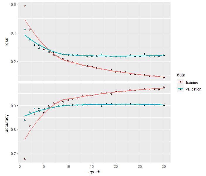
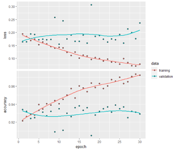
We end up with a Training accuracy = 97.25% and Validation accuracy = 92.90%. This model clearly outperforms the previous ones. If we increase the epochs we can observe the network achieving higher accuracy.
What if the Loss curve doesn’t show any real improvement ?
What is displayed in the graphs is an average of point-wise loss values; but what matters for accuracy is the distribution of the loss values, not their average, because accuracy is the result of a binary thresholding of the class probability predicted by the model. The model may still be improving even if this isn’t reflected in the average loss.
Let’s Evaluate !
Code
model %>%evaluate_generator(test_generator, steps =50)
We arrive at a Test accuracy = 93.5%!
To Summarise,
Model
Network Structure
Training Accuracy
Validation Accuracy
Test Accuracy
1
4 conv_layers with (32, 64, 128, 128) and one dense_layer 512 hidden units
98.35 %
71.10 %
-
2
4 conv_layers with (32, 64, 128, 128) and two dense_layers with (512, 46) hidden units. 50% Dropout.
(with Data Augmentation)
82.50 %
76.20 %
-
3
vgg16 (Fast Feature Extraction without Data Augmentation)
97.70 %
90.1 %
-
4
vgg16 (Feature Extraction with Data Augmentation)
87.70 %
90.80 %
-
5
vgg16 (Fine Tuning) ***
97.25 %
92.90 %
93.5 %
Let’s now visualise how these networks learn these patterns !